Introduction

Physical quantities described by just a number: scalars

Physical quantities described by a number and a direction: vectors

More generally, vectors can represent a collection of ordered numbers

$$\mathbf{v} = (v_{1}, v_{2}, \ldots , v_{n})$$

Introduction

Vectors are very useful in physics to deal with concepts such as force, speed, fields, etc.

They are also useful to the treatment of data in general

Example: the cosine of the angle between two vectors is often used in text analysis to determine the similarity between documents

Basic Operations

A number of basic operations can be applied to vectors:

  → Addition

  → Subtraction

  → Multiplication by a scalar

Vector Operations

Additionaly, we can define:

  → The norm of a vector

  → The angle between two vectors

  → The dot product of two vectors

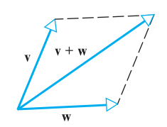
Addition

$$\mathbf{v} + \mathbf{w} = (v_{1} + w_{1}, v_{2} + w_{2}, \ldots , v_{n} + w_{n})$$

Subtraction

$$\mathbf{w} - \mathbf{v} = \mathbf{w} + (- \mathbf{v}) = (w_{1} - v_{1}, w_{2} - v_{2}, \ldots , w_{n} - v_{n})$$

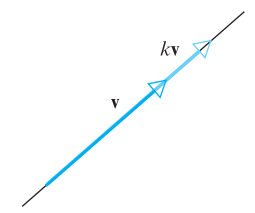
Multiplication by a Scalar

$$k\mathbf{v} = (kv_{1}, kv_{2}, \ldots , kv_{n})$$

Properties

Basic Operations on vectors follow these properties:

  → Commutative

  → Associative

  → Distributive (over a scalar)

  → Identities (scalar and vector)

Norm

The norm of a vector is a measure of its length

It is represented by:

$$||\mathbf{v}||$$

And, it can calculated as:

$$||\mathbf{v}|| = \sqrt{ v_{1}^{2} + v_{2}^{2} + \ldots + v_{n}^{2} }$$

Norm properties

The norm of a vector follows these properties:

$$||\mathbf{v}|| \geq 0$$

$$||\mathbf{v}|| = 0\ \text{if and only if}\ \mathbf{v} = \mathbf{0}$$

$$||k\mathbf{v}|| = |k|||\mathbf{v}||$$

Normalizing Vectors

A vector of norm 1 is called a unit vector

Vectors can be normalized:

$$\mathbf{u} = \frac{\mathbf{v}}{||\mathbf{v}||}$$

A vector with a 1 in one position, and zeroes elsewhere is a standard unit vector

Any vector can be written as a linear combination of standard unit vectors

Distance

The distance between two vectors is defined as

$$d (\mathbf{u}, \mathbf{v}) = ||\mathbf{u} - \mathbf{v}||$$

$$= \sqrt{ (u_{1} - v_{1})^{2} + (u_{2} - v_{2})^{2} + \ldots + (u_{n} - v_{n})^{2} }$$

Dot Product

The dot product of vectors u and v is defined as:

$$\mathbf{u} \cdot \mathbf{v} = ||\mathbf{u}||||\mathbf{v}||\cos{\theta}$$

Therefore, cos(θ), can be calculated as:

$$\frac{\mathbf{u} \cdot \mathbf{v}}{||\mathbf{u}||||\mathbf{v}||}$$

Dot Product

Using the law of cosines, one can show that:

$$\mathbf{u} \cdot \mathbf{v} = 0.5(||\mathbf{u}||^{2} + ||\mathbf{v}||^{2}- ||\mathbf{u - v}||^{2})$$

$$\mathbf{u} \cdot \mathbf{v} = u_{1}v_{1} + u_{2}v_{2} + \ldots + u_{n}v_{n}$$

Dot Product Properties

The dot product follows these properties:

$$\mathbf{u} \cdot \mathbf{v} = \mathbf{v} \cdot \mathbf{u}$$

$$\mathbf{u} \cdot ( \mathbf{v} + \mathbf{w})= \mathbf{v} \cdot \mathbf{u} + \mathbf{v} \cdot \mathbf{w}$$

$$k(\mathbf{u} \cdot \mathbf{v}) = (k\mathbf{u}) \cdot \mathbf{v}$$

$$\mathbf{v} \cdot \mathbf{v} \geq 0\ \text{, and}\ \mathbf{v} \cdot \mathbf{v} = 0\ \text{if and only if}\ \mathbf{v} = \mathbf{0}$$

Introduction

Previously, we showed that two points represent a line in a plane

One can also show that a point and a vector also represent a line

$$\mathbf{x} = \mathbf{x}_{0} + k\mathbf{v}$$

Introduction

The same way, a point and two vectors represent a plane in a 3D space

$$\mathbf{x} = \mathbf{x}_{0} + k_{1}\mathbf{v}_{1} + k_{2}\mathbf{v}_{2}$$

Parametric Equations

Given an equation of the type:

$$ax + by + cz = d$$

One can find its vector parametric equations as:

$$x = \frac{1}{a}(d - bt_{1} - ct_{2}),\ y = t_{1},\ z = t_{2}$$

Parametric Equations

So, we have:

$$(x, y, z) = (\frac{1}{a}(d - bt_{1} - ct_{2}), \frac{1}{a}t_{1}, \frac{1}{a}t_{2})$$

Or, conversely:

$$(x, y, z) = (\frac{d}{a}, 0, 0) + t_{1}(-\frac{b}{a}, \frac{1}{a}, 0) + t_{2}(-\frac{c}{a}, 0, \frac{1}{a})$$

Dot Product of Linear Systems

A linear equation such as:

$$a_{1}x_{1} + a_{2}x_{2} + \ldots + a_{n}x_{n} = b$$

Can be rewriten in dot product as:

$$\mathbf{x}\cdot \mathbf{a} = b,$$

$$\text{where}\ \mathbf{x} = (x_{1}, x_{2}, \ldots, x_{n})\ \text{and}\ \mathbf{a} = (a_{1}, a_{2}, \ldots, a_{n})$$

Dot Product of Linear Systems

For a homogeneous system of equations:

$$\begin{aligned} a_{11}x_{1} & + a_{12}x_{2} & + \cdots + & a_{1n}x_{n} & = 0 \\ a_{21}x_{1} & + a_{22}x_{2} & + \cdots + & a_{2n}x_{n} & = 0 \\ \vdots & + \vdots & + \cdots + & \vdots& = \vdots \\ a_{m1}x_{1} & + a_{m2}x_{2} & + \cdots + & a_{mn}x_{n} & = 0 \end{aligned}$$

Dot Product of Linear Systems

We can rewrite it as:

$$\begin{aligned} \mathbf{r}_{1}\cdot\mathbf{x} & = 0 \\ \mathbf{r}_{2}\cdot\mathbf{x} & = 0 \\ \vdots & = \vdots \\ \mathbf{r}_{m}\cdot\mathbf{x} & = 0 \end{aligned}$$

Dot Product of Linear Systems

This means that every possible solution x is orthogonal to each vector r

Example

$$\begin{bmatrix} 1 & 2 & -1 \\ 1 & 0 & -1 \\ 2 & 2 & 0 \\ \end{bmatrix} \begin{bmatrix} x_{0} \\ x_{1} \\ x_{2} \\ \end{bmatrix} = \begin{bmatrix} 0 \\ 0 \\ 0 \\ \end{bmatrix}$$

Solution

$$(x_{0}, x_{1}, x_{2}) = t(1,0,0) - t(0,1,0) + t(0, 0, 1)$$

Dot Product of Linear Systems

The solution of each non-homogeneous system is equal to that of a homogeneous systems plus a fixed vector

Example

$$\begin{bmatrix} 1 & 2 & -1 \\ 1 & 0 & -1 \\ 2 & 2 & 0 \\ \end{bmatrix} \begin{bmatrix} x_{0} \\ x_{1} \\ x_{2} \\ \end{bmatrix} = \begin{bmatrix} 1 \\ 1 \\ 1 \\ \end{bmatrix}$$

Solution

$$(x_{0}, x_{1}, x_{2}) = (1, 0 , 0) + t(1,0,0) - t(0,1,0) + t(0, 0, 1)$$